Data Modeling & Tidy Data
Learning Objectives
- Understand basics of relational data models aka tidy data
- Learn how to design and create effective data tables
Benefits of relational data systems
- Powerful search and filtering
- Handle large, complex data sets
- Enforce data integrity
- Decrease errors from redundant updates
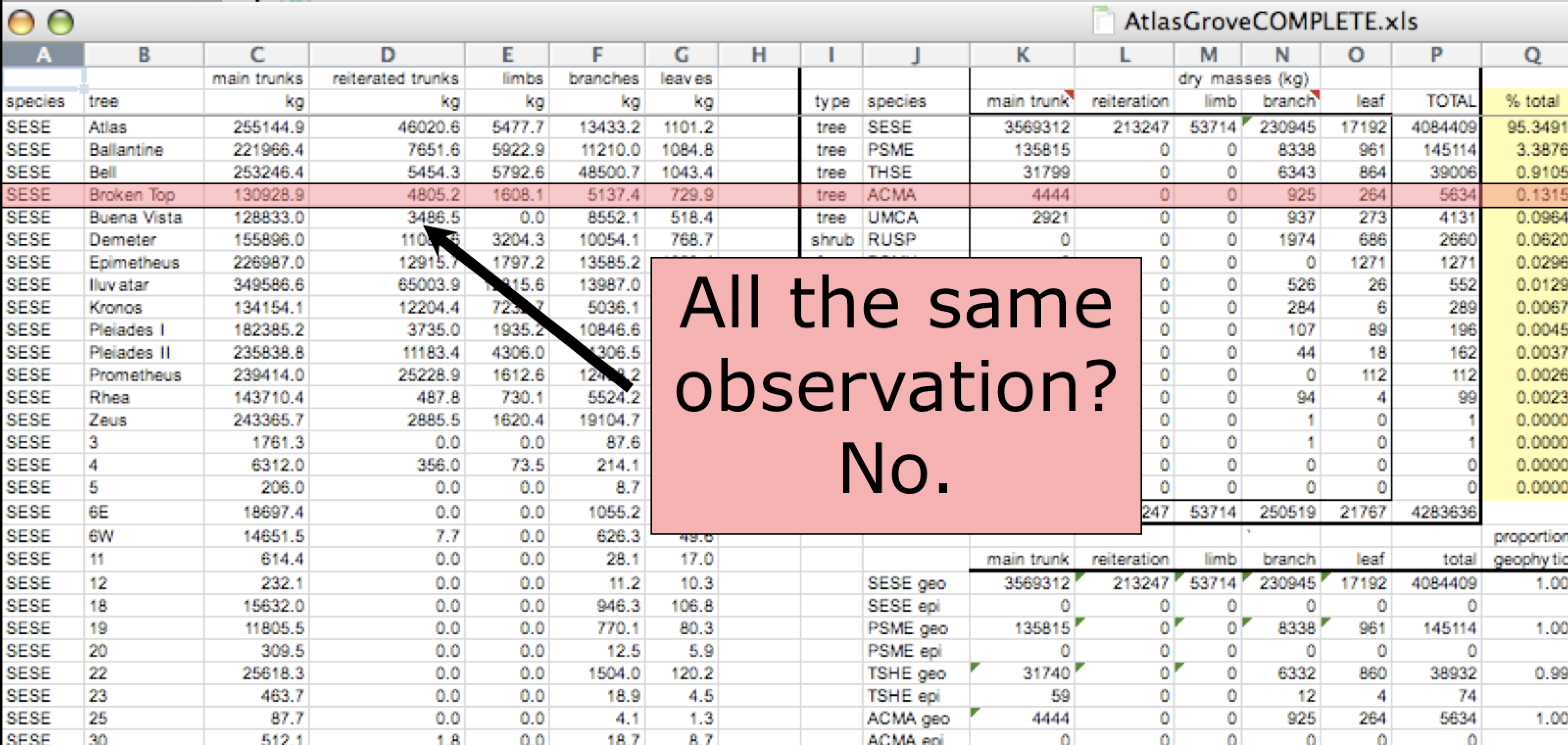
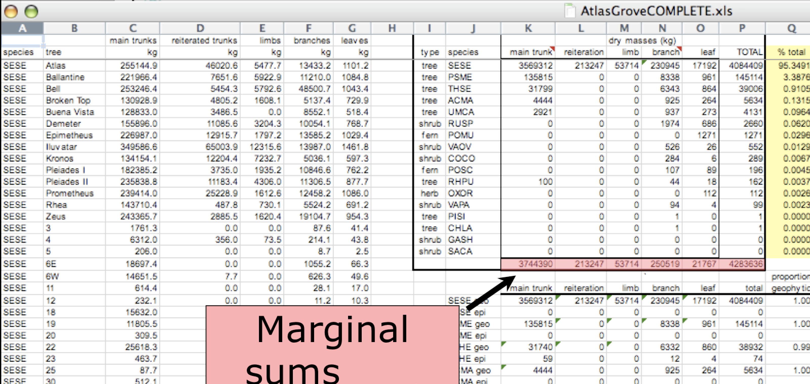
Inconsistent observations
Marginal sums and statistics
Good enough data modeling
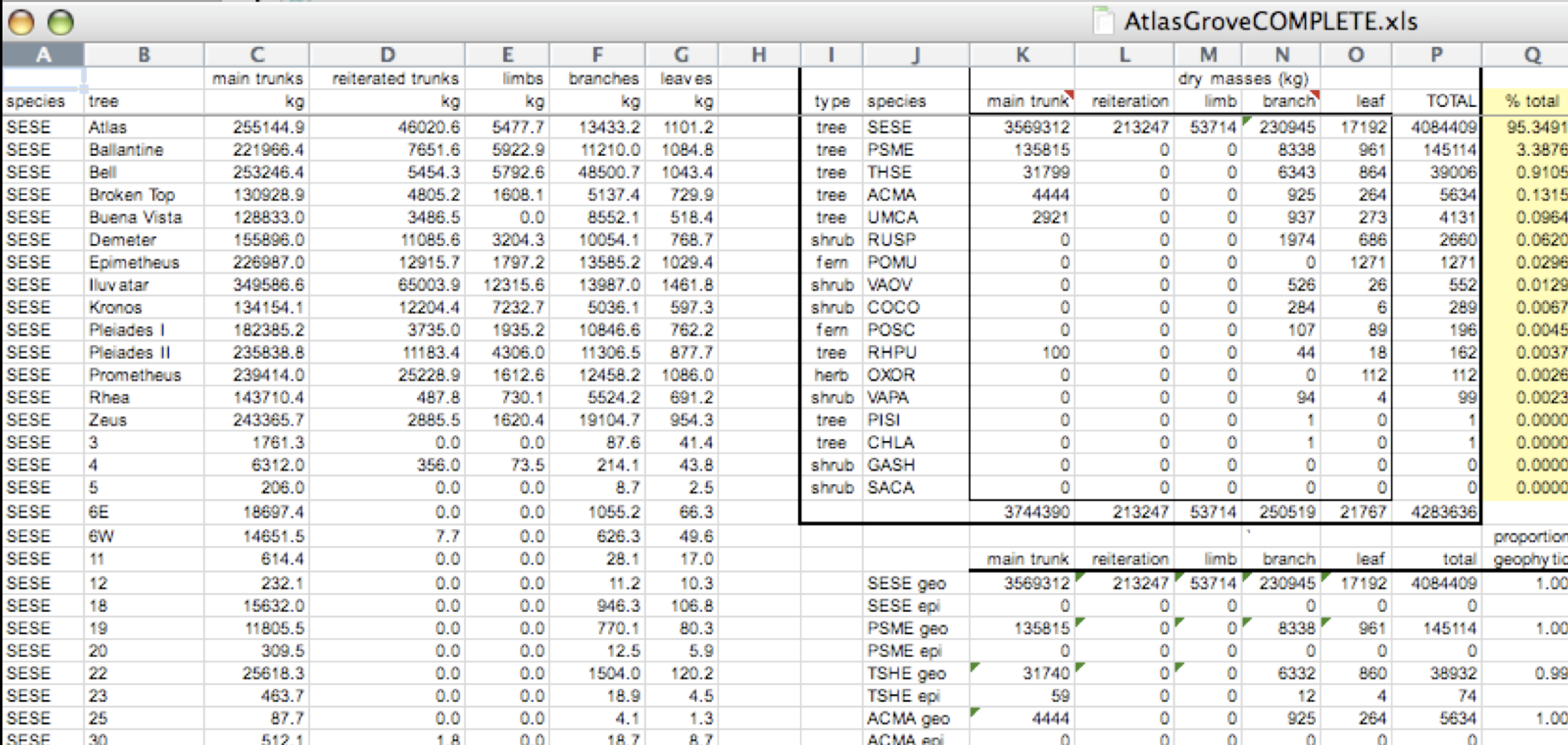
Denormalized data
- Observations about different entities combined
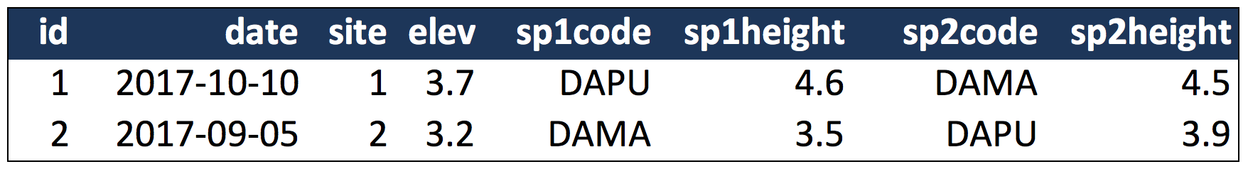 In the above example, each row has measurements about both the
 site at which observations occurred, as well as observations of two individuals of possibly different species found at that site. This is not normalized data.
People often refer to this as wide format, because the observations are spread across a wide number of columns. Note that, should one encounter a new species in the survey, we wold have to add new columns to the table. This is difficult to analyze, understand, and maintain.
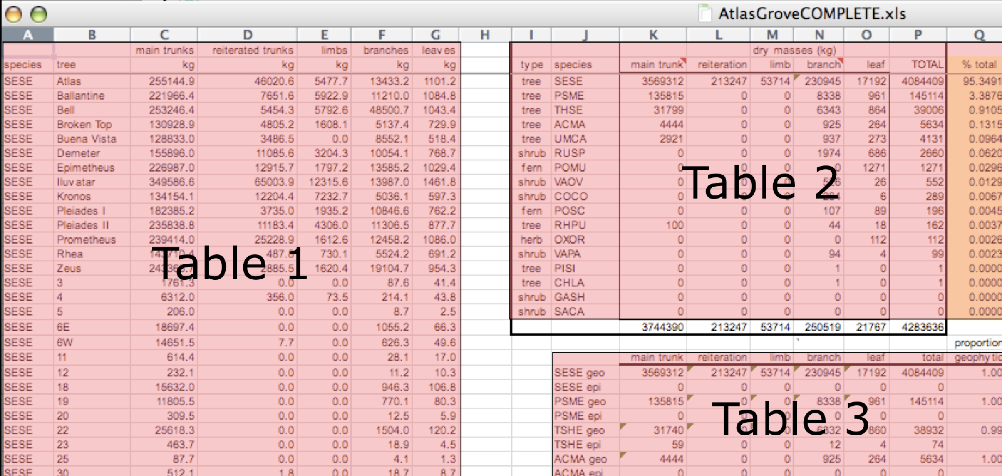
Tabular data
Observations. A better way to model data is to organize the observations about each type of entity in its own table. This results in:
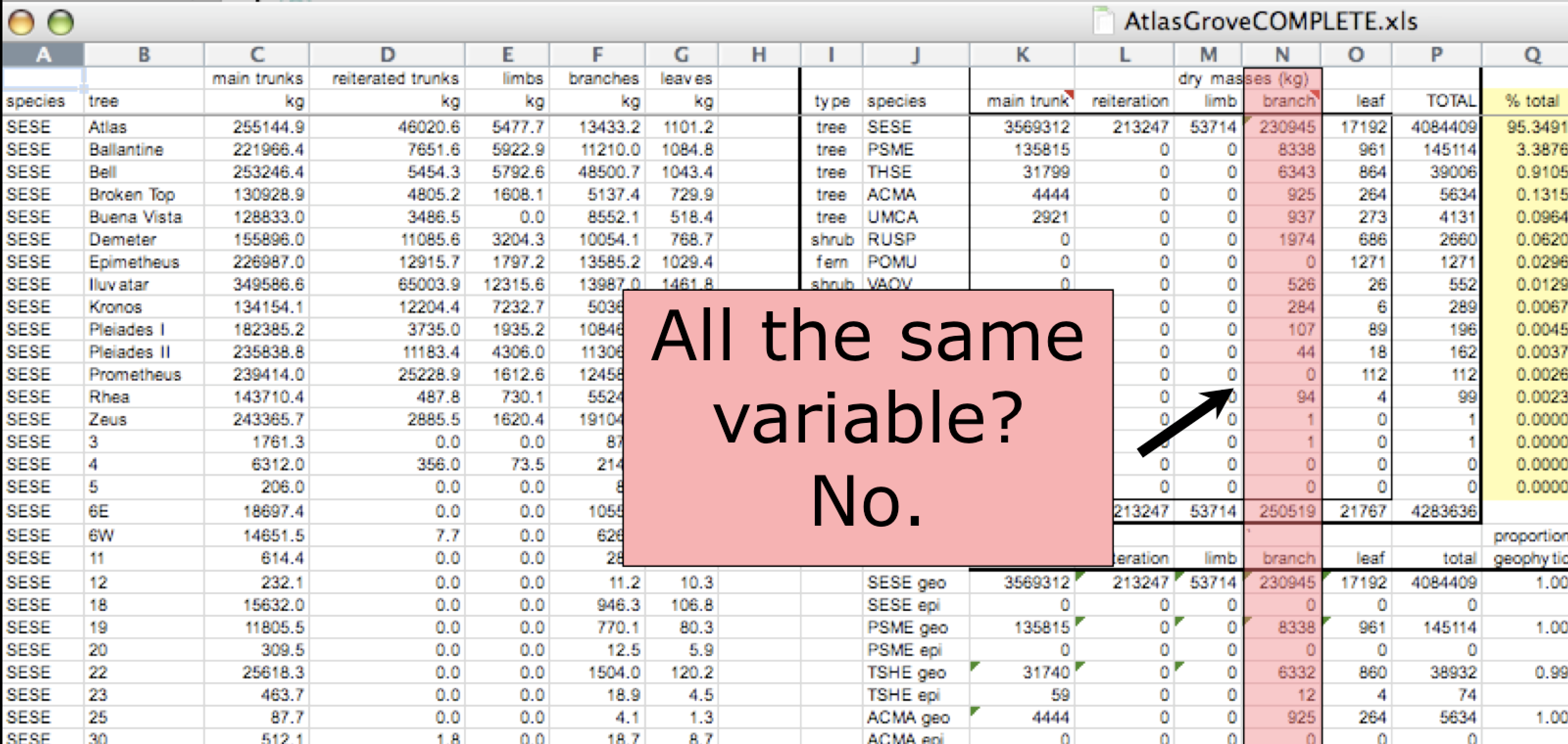
Variables. In addition, for normalized data, we expect the variables to be organized such that:
- All values in a column are of the same type
- All columns pertain to the same observed entity (e.g., row)
- Each column represents either an identifying variable or a measured variable
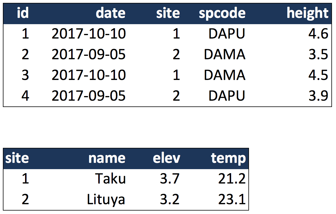
Here’s an example of tidy (normalized) data in which the top table is the collection of observations about individuals of several species, and the bottom table are the observations containing properties of the sites at which the species occurred.
Primary and Foreign Keys
When one has normalized data, we often use unique identifiers to reference particular observations, which allows us to link across tables. Two types of identifiers are common within relational data:
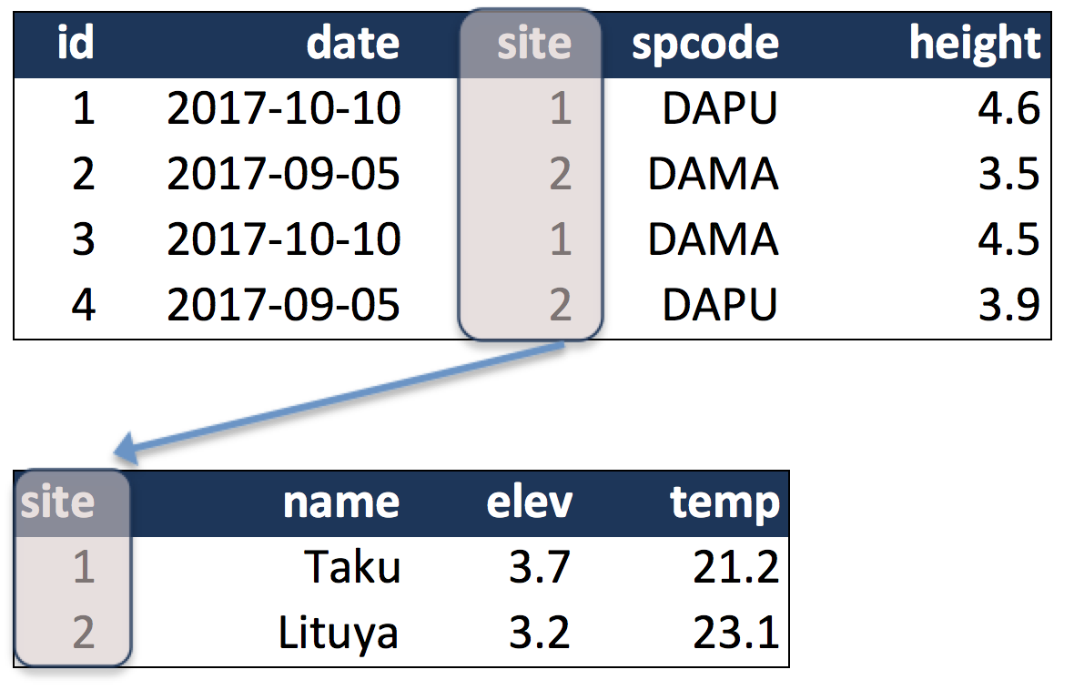
- Primary Key: unique identifier for each observed entity, one per row
- Foreign Key: reference to a primary key in another table (linkage)
For example, in the second table below, the site column is the primary key of that table, because it uniquely identifies each row of the table as a unique observation of a site. Inthe first table, however, the site column is a foreign key that references the primary key from the second table. This linkage tells us that the first height measurement for the DAPU observation occurred at the site with the name Taku.
Entity-Relationship Model (ER)
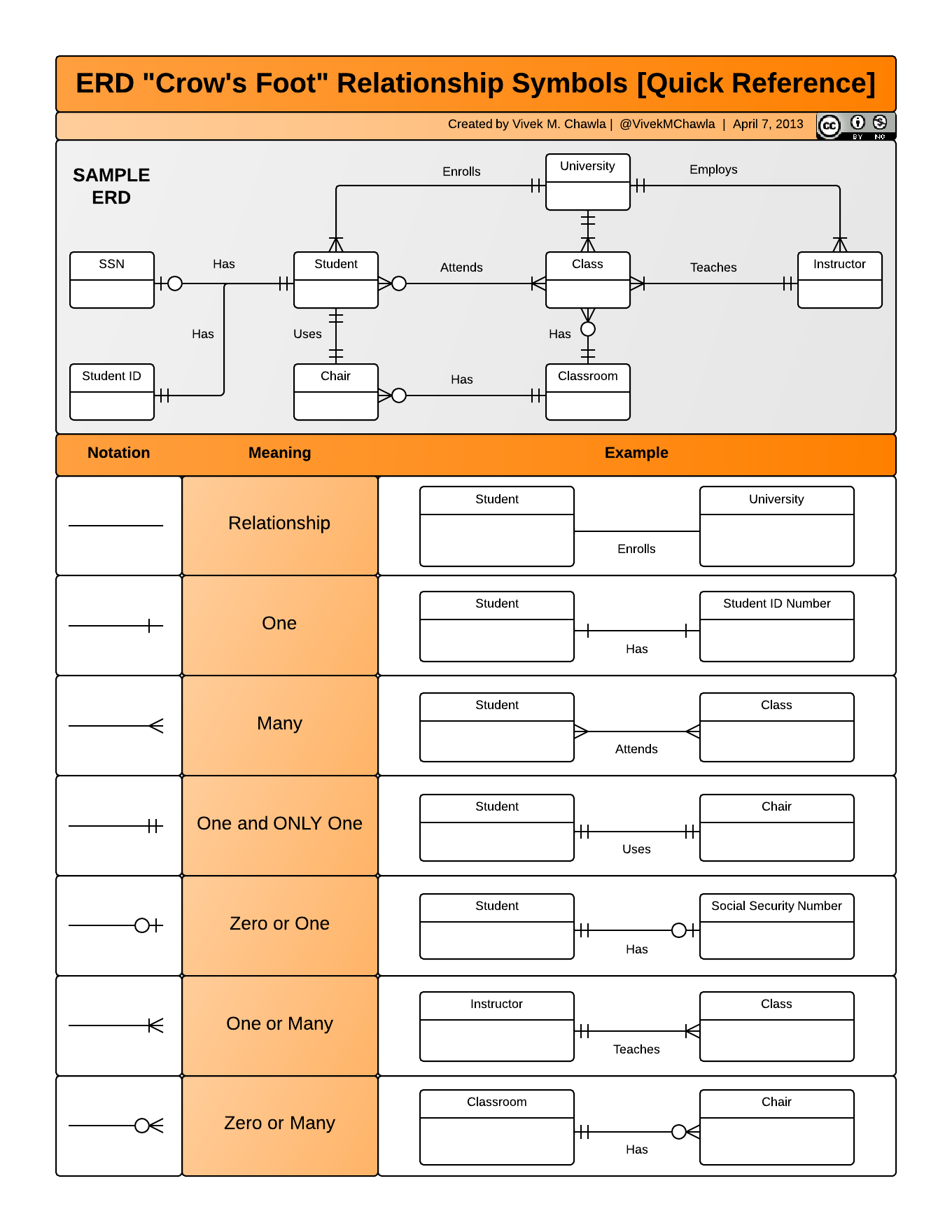
An Entity-Relationship model allows us to compactly draw the structure of the tables in a relational database, including the primary and foreign keys in the tables.
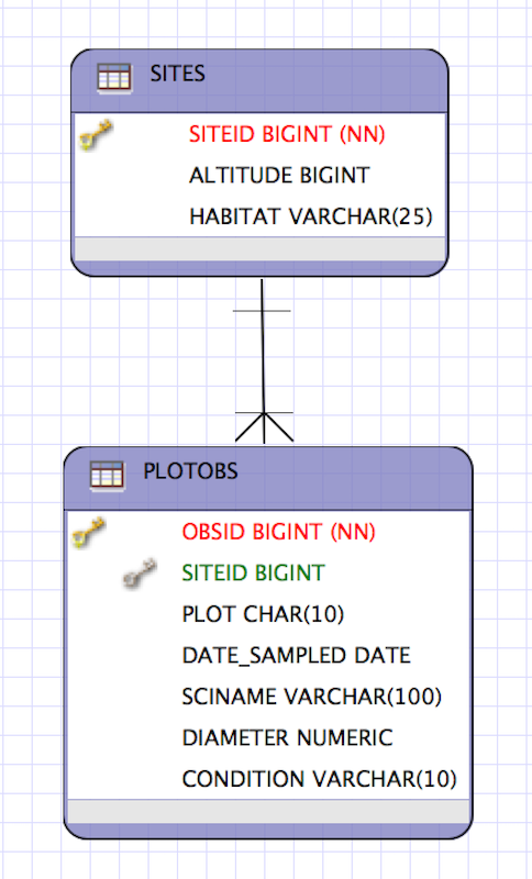 In the above model, one can see that each site in the
 SITES table must have one or more observations in the PLOTOBS table, whereas each PLOTOBS has one and only one SITE.
Merging data
Frequently, analysis of data will require merging these separately managed tables back together. There are multiple ways to join the observations in two tables, based on how the rows of one table are merged with the rows of the other.
When conceptualizing merges, one can think of two tables, one on the left and one on the right. The most common (and often useful) join is when you merge the subset of rows that have matches in both the left table and the right table: this is called an INNER JOIN. Other types of join are possible as well. A LEFT JOIN takes all of the rows from the left table, and merges on the data from matching rows in the right table. A RIGHT JOIN is the same, except that all of the rows from the right table are included with matching data from the left. Finally, a FULL OUTER JOIN includes all data from all rows in both tables (and is rarely practical).
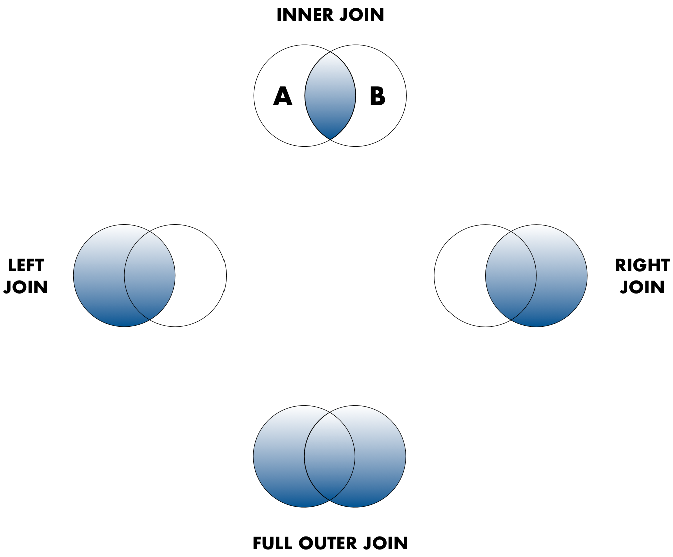 In the figure above, the blue regions show the set of rows that are included in the result. For the INNER join, the rows returned are all rows in A that have a matching row in B.
Simple Guidelines for Effective Data
Data modeling exercise
- Break into groups, 1 per table
To demonstrate, we’ll be working with a tidied up version of a dataset from ADF&G containing commercial catch data from 1878-1997. The dataset and reference to the original source can be viewed at its public archive: https://knb.ecoinformatics.org/#view/df35b.304.2. That site includes metadata describing the full data set, including column definitions. Here’s the first catch table:
And here’s the region_defs table:
- Draw an ER model for the tables
- Indicate the primary and foreign keys
- Is the
catch table in normal (aka tidy) form?
- If so, what single type of entity was observed?
- If not, how might you restructure the data table to make it tidy?
- Draw a new ER diatram showing this re-designed data structure