11 Data Cleaning and Manipulation
11.1 Learning Objectives
In this lesson, you will learn:
- What the Split-Apply-Combine strategy is and how it applies to data
- The difference between wide vs. tall table formats and how to convert between them
- How to use
dplyrandtidyrto clean and manipulate data for analysis - How to join multiple
data.frames together usingdplyr
11.2 Introduction
The data we get to work with are rarely, if ever, in the format we need to do our analyses. It’s often the case that one package requires data in one format, while another package requires the data to be in another format. To be efficient analysts, we should have good tools for reformatting data for our needs so we can do our actual work like making plots and fitting models. The dplyr and tidyr R packages provide a fairly complete and extremely powerful set of functions for us to do this reformatting quickly and learning these tools well will greatly increase your efficiency as an analyst.
Analyses take many shapes, but they often conform to what is known as the Split-Apply-Combine strategy. This strategy follows a usual set of steps:
- Split: Split the data into logical groups (e.g., area, stock, year)
- Apply: Calculate some summary statistic on each group (e.g. mean total length by year)
- Combine: Combine the groups back together into a single table
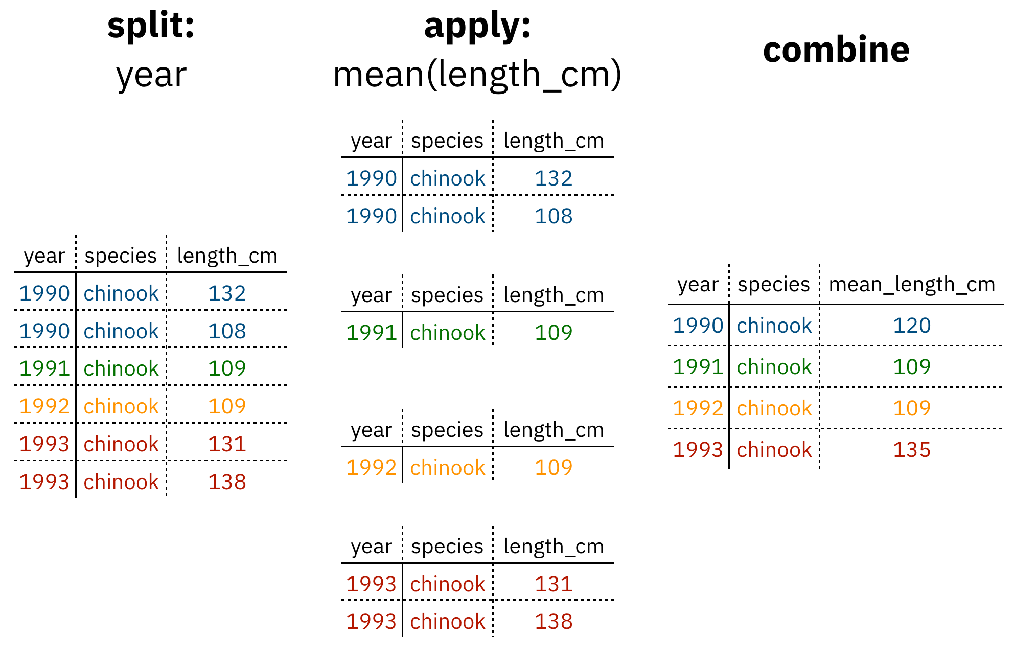
Figure 1: diagram of the split apply combine strategy
As shown above (Figure 1), our original table is split into groups by year, we calculate the mean length for each group, and finally combine the per-year means into a single table.
dplyr provides a fast and powerful way to express this. Let’s look at a simple example of how this is done:
Assuming our length data is already loaded in a data.frame called length_data:
| year | length_cm |
|---|---|
| 1991 | 5.673318 |
| 1991 | 3.081224 |
| 1991 | 4.592696 |
| 1992 | 4.381523 |
| 1992 | 5.597777 |
| 1992 | 4.900052 |
| 1992 | 4.139282 |
| 1992 | 5.422823 |
| 1992 | 5.905247 |
| 1992 | 5.098922 |
We can do this calculation using dplyr like this:
length_data %>%
  group_by(year) %>%
  summarise(mean_length_cm = mean(length_cm))
Another exceedingly common thing we need to do is “reshape” our data. Let’s look at an example table that is in what we will call “wide” format:
| site | 1990 | 1991 | … | 1993 |
|---|---|---|---|---|
| gold | 100 | 118 | … | 112 |
| lake | 100 | 118 | … | 112 |
| … | … | … | … | … |
| dredge | 100 | 118 | … | 112 |
You are probably quite familiar with data in the above format, where values of the variable being observed are spread out across columns (Here: columns for each year). Another way of describing this is that there is more than one measurement per row. This wide format works well for data entry and sometimes works well for analysis but we quickly outgrow it when using R. For example, how would you fit a model with year as a predictor variable? In an ideal world, we’d be able to just run:
lm(length ~ year)But this won’t work on our wide data because lm needs length and year to be columns in our table.
Or how would we make a separate plot for each year? We could call plot one time for each year but this is tedious if we have many years of data and hard to maintain as we add more years of data to our dataset.
The tidyr package allows us to quickly switch between wide format and what is called tall format using the gather function:
site_data %>%
gather(year, length, -site)| site | year | length |
|---|---|---|
| gold | 1990 | 101 |
| lake | 1990 | 104 |
| dredge | 1990 | 144 |
| … | … | … |
| dredge | 1993 | 145 |
In this lesson we’re going to walk through the functions you’ll most commonly use from the dplyr and tidyr packages:
dplyrmutate()group_by()summarise()select()filter()arrange()left_join()rename()
tidyrgather()spread()extract()separate()
11.3 Setup
Let’s start going over the most common functions you’ll use from the dplyr package. To demonstrate, we’ll be working with a tidied up version of a dataset from ADF&G containing commercial catch data from 1878-1997. The dataset and reference to the original source can be found at its public archive: https://knb.ecoinformatics.org/#view/df35b.304.2.
First, let’s load dplyr and tidyr:
library(dplyr)
library(tidyr)
Then let’s read in the data and take a look at it:
catch_original <- read.csv(url("https://knb.ecoinformatics.org/knb/d1/mn/v2/object/df35b.302.1", method = "libcurl"),
                    stringsAsFactors = FALSE)
head(catch_original)
## Region Year Chinook Sockeye Coho Pink Chum All notesRegCode
## 1 SSE 1886 0 5 0 0 0 5
## 2 SSE 1887 0 155 0 0 0 155
## 3 SSE 1888 0 224 16 0 0 240
## 4 SSE 1889 0 182 11 92 0 285
## 5 SSE 1890 0 251 42 0 0 292
## 6 SSE 1891 0 274 24 0 0 298Note: I copied the URL from the Download button on https://knb.ecoinformatics.org/#view/df35b.304.2
This dataset is relatively clean and easy to interpret as-is. But while it may be clean, it’s in a shape that makes it hard to use for some types of analyses so we’ll want to fix that first.
11.4 About the pipe (%>%) operator
Before we jump into learning tidyr and dplyr, we first need to explain the %>%.
Both the tidyr and the dplyr packages use the pipe operator - %>%, which may look unfamiliar. The pipe is a powerful way to efficiently chain together operations. The pipe will take the output of a previous statement, and use it as the input to the next statement.
Say you want to both filter out rows of a dataset, and select certain columns. Instead of writing
df_filtered <- filter(df, ...)
df_selected <- select(df_filtered, ...)
You can write
df_cleaned <- df %>%
              filter(...) %>%
              select(...)
If you think of the assignment operator (<-) as reading like “gets”, then the pipe operator would read like “then.”
So you might think of the above chunk being translated as:
The cleaned dataframe gets the original data, and then a filter (of the original data), and then a select (of the filtered data).
The benefits to using pipes are that you don’t have to keep track of (or overwrite) intermediate data frames. The drawbacks are that it can be more difficult to explain the reasoning behind each step, especially when many operations are chained together. It is good to strike a balance between writing efficient code (chaining operations), while ensuring that you are still clearly explaining, both to your future self and others, what you are doing and why you are doing it.
RStudio has a keyboard shortcut for %>% : Ctrl + Shift + M (Windows), Cmd + Shift + M (Mac).
11.5 Selecting/removing columns: select()
The first issue is the extra columns All and notesRegCode. Let’s select only the columns we want, and assign this to a variable called catch_data.
catch_data <- catch_original %>%
  select(Region, Year, Chinook, Sockeye, Coho, Pink, Chum)

head(catch_data)
## Region Year Chinook Sockeye Coho Pink Chum
## 1 SSE 1886 0 5 0 0 0
## 2 SSE 1887 0 155 0 0 0
## 3 SSE 1888 0 224 16 0 0
## 4 SSE 1889 0 182 11 92 0
## 5 SSE 1890 0 251 42 0 0
## 6 SSE 1891 0 274 24 0 0Much better!
select also allows you to say which columns you don’t want, by passing unquoted column names preceded by minus (-) signs:
catch_data <- catch_original %>%
  select(-All, -notesRegCode)

head(catch_data)
## Region Year Chinook Sockeye Coho Pink Chum
## 1 SSE 1886 0 5 0 0 0
## 2 SSE 1887 0 155 0 0 0
## 3 SSE 1888 0 224 16 0 0
## 4 SSE 1889 0 182 11 92 0
## 5 SSE 1890 0 251 42 0 0
## 6 SSE 1891 0 274 24 0 011.6 Changing shape: gather() and spread()
The next issue is that the data are in a wide format and, we want the data in a tall format instead. gather() from the tidyr package helps us do just this conversion:
catch_long <- catch_data %>%
  gather(species, catch, -Region, -Year)

head(catch_long)
## Region Year species catch
## 1 SSE 1886 Chinook 0
## 2 SSE 1887 Chinook 0
## 3 SSE 1888 Chinook 0
## 4 SSE 1889 Chinook 0
## 5 SSE 1890 Chinook 0
## 6 SSE 1891 Chinook 0The syntax we used above for gather() might be a bit confusing so let’s look at an annotated diagram:
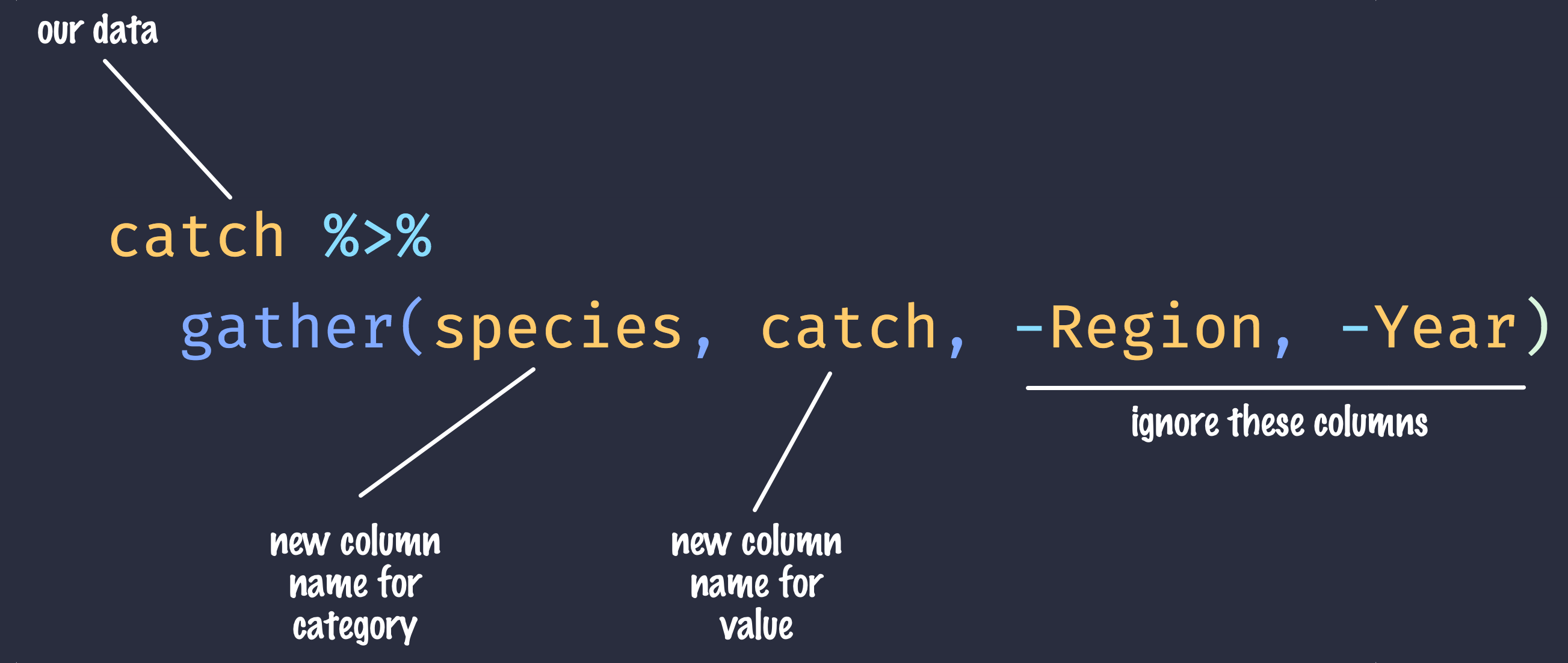
annotated gather code
The first two arguments to gather() are the names of new columns that will be created and the other arguments with - symbols in front of them are columns to keep around in this process. The opposite of gather(), spread(), works in a similar declarative fashion:
catch_wide <- catch_long %>%
  spread(species, catch)

head(catch_wide)
## Region Year Chinook Chum Coho Pink Sockeye
## 1 ALU 1911 0 0 0 0 9
## 2 ALU 1912 0 0 0 0 0
## 3 ALU 1913 0 0 0 0 0
## 4 ALU 1914 0 0 0 0 0
## 5 ALU 1915 0 0 0 0 0
## 6 ALU 1916 0 0 1 180 7611.7 Renaming columns with rename()
If you scan through the data, you may notice the values in the catch column are very small (these are supposed to be annual catches). If we look at the metadata we can see that the catch column is in thousands of fish so let’s convert it before moving on.
Let’s first rename the catch column to be called catch_thousands:
catch_clean <- catch_long %>%
  rename(catch_thousands = catch)

head(catch_clean)
## Region Year species catch_thousands
## 1 SSE 1886 Chinook 0
## 2 SSE 1887 Chinook 0
## 3 SSE 1888 Chinook 0
## 4 SSE 1889 Chinook 0
## 5 SSE 1890 Chinook 0
## 6 SSE 1891 Chinook 011.8 Adding columns: mutate()
Now let’s create a new column called catch with units of fish (instead of thousands of fish). Note that here we have added to the expression we wrote above by adding another function call (mutate) to our expression. This takes advantage of the pipe operator by grouping together a similar set of statements, which all aim to clean up the catch_long data.frame.
catch_clean <- catch_long %>%
  rename(catch_thousands = catch) %>%
  mutate(catch = catch_thousands * 1000)

head(catch_clean)
You’ll notice that we get an error:
Error in mutate_impl(.data, dots) : Evaluation error: non-numeric argument to binary operator.
This is an extremely cryptic error – what is it telling us? These kinds of errors can be very hard to diagnose, but maybe the catch column isn’t quite what we are expecting. How could we find out? R provides a number of handy utility functions for quickly summarizing a large table:
summary(catch_clean)## Region Year species catch_thousands
## Length:8540 Min. :1878 Length:8540 Length:8540
## Class :character 1st Qu.:1922 Class :character Class :character
## Mode :character Median :1947 Mode :character Mode :character
## Mean :1946
## 3rd Qu.:1972
## Max. :1997- Exercise: What are some other ways (functions) we could’ve found out what our problem was?
Notice in the above output that the catch_thousands column shows up as Class :character. That seems wrong since catch should be whole numbers (in R, these show up as integers).
Let’s try to convert the values to integers and see what happens:
catch_integers <- as.integer(catch_clean$catch_thousands)## Warning: NAs introduced by coercionWe get an error “NAs introduced by coercion” which is R telling us that it couldn’t convert every value to an integer and, for those values it couldn’t convert, it put an NA in its place. This is behavior we commonly experience when cleaning datasets and it’s important to have the skills to deal with it when it crops up. We can find out which values are NAs with a combination of is.na() and which(), and save that to a variable called i.
i <- which(is.na(catch_integers))
i
## [1] 401It looks like there is only one problem row, lets have a look at it:
catch_clean[i,]## Region Year species catch_thousands
## 401 GSE 1955 Chinook IWell that’s odd: The value in catch_thousands is I which is isn’t even a number. It turns out that this dataset is from a PDF which was automatically converted into a CSV and this value of I is actually a 1. Let’s fix it:
catch_clean <- catch_long %>%
  rename(catch_thousands = catch) %>%
  mutate(catch_thousands = ifelse(catch_thousands == "I", 1, catch_thousands)) %>%
  mutate(catch_thousands = as.integer(catch_thousands))

head(catch_clean)
## Region Year species catch_thousands
## 1 SSE 1886 Chinook 0
## 2 SSE 1887 Chinook 0
## 3 SSE 1888 Chinook 0
## 4 SSE 1889 Chinook 0
## 5 SSE 1890 Chinook 0
## 6 SSE 1891 Chinook 0Note that, in the above pipeline call to mutate(), we mutate catch_thousands twice. This works because mutate() processes each of the mutations in a step-wise fashion so the results of one mutation are available for the next.
Now let’s try our conversion again by adding it as another function call in our expression.
catch_clean <- catch_long %>%
  rename(catch_thousands = catch) %>%
  mutate(catch_thousands = ifelse(catch_thousands == "I", 1, catch_thousands)) %>%
  mutate(catch_thousands = as.integer(catch_thousands)) %>%
  mutate(catch = catch_thousands * 1000)

head(catch_clean)
## Region Year species catch_thousands catch
## 1 SSE 1886 Chinook 0 0
## 2 SSE 1887 Chinook 0 0
## 3 SSE 1888 Chinook 0 0
## 4 SSE 1889 Chinook 0 0
## 5 SSE 1890 Chinook 0 0
## 6 SSE 1891 Chinook 0 0Looks good, no warnings! Now let’s remove the catch_thousands column for now since we don’t need it:
catch_clean <- catch_long %>%
  rename(catch_thousands = catch) %>%
  mutate(catch_thousands = ifelse(catch_thousands == "I", 1, catch_thousands)) %>%
  mutate(catch_thousands = as.integer(catch_thousands)) %>%
  mutate(catch = catch_thousands * 1000) %>%
  select(-catch_thousands)

head(catch_clean)
## Region Year species catch
## 1 SSE 1886 Chinook 0
## 2 SSE 1887 Chinook 0
## 3 SSE 1888 Chinook 0
## 4 SSE 1889 Chinook 0
## 5 SSE 1890 Chinook 0
## 6 SSE 1891 Chinook 0We’re now ready to start analyzing the data.
11.9 group_by and summarise
As I outlined in the Introduction, dplyr lets us employ the Split-Apply-Combine strategy and this is exemplified through the use of the group_by() and summarise() functions:
mean_region <- catch_clean %>%
  group_by(Region) %>%
  summarise(mean(catch))

head(mean_region)
## # A tibble: 6 x 2
## Region `mean(catch)`
## <chr> <dbl>
## 1 ALU 40384.
## 2 BER 16373.
## 3 BRB 2709796.
## 4 CHG 315487.
## 5 CKI 683571.
## 6 COP 179223.- Exercise: Find another grouping and statistic to calculate for each group.
- Exercise: Find out if you can group by multiple variables.
Another common use of group_by() followed by summarize() is to count the number of rows in each group. We have to use a special function from dplyr, n().
n_region <- catch_clean %>%
  group_by(Region) %>%
  summarize(n = n())

head(n_region)
## # A tibble: 6 x 2
## Region n
## <chr> <int>
## 1 ALU 435
## 2 BER 510
## 3 BRB 570
## 4 CHG 550
## 5 CKI 525
## 6 COP 47011.10 Filtering rows: filter()
filter() is the verb we use to filter our data.frame to rows matching some condition. It’s similar to subset() from base R.
Let’s go back to our original data.frame and do some filter()ing:
SSE_catch <- catch_clean %>%
  filter(Region == "SSE")

head(SSE_catch)
## Region Year species catch
## 1 SSE 1886 Chinook 0
## 2 SSE 1887 Chinook 0
## 3 SSE 1888 Chinook 0
## 4 SSE 1889 Chinook 0
## 5 SSE 1890 Chinook 0
## 6 SSE 1891 Chinook 0- Exercise: Filter to just catches of over one million fish.
- Exercise: Filter to just SSE Chinook
11.11 Sorting your data: arrange()
arrange() is how we sort the rows of a data.frame. In my experience, I use arrange() in two common cases:
- When I want to calculate a cumulative sum (with
cumsum()) so row order matters - When I want to display a table (like in an
.Rmddocument) in sorted order
Let’s re-calculate mean catch by region, and then arrange() the output by mean catch:
mean_region <- catch_clean %>%
  group_by(Region) %>%
  summarise(mean_catch = mean(catch)) %>%
  arrange(mean_catch)

head(mean_region)
## # A tibble: 6 x 2
## Region mean_catch
## <chr> <dbl>
## 1 BER 16373.
## 2 KTZ 18836.
## 3 ALU 40384.
## 4 NRS 51503.
## 5 KSK 67642.
## 6 YUK 68646.The default sorting order of arrange() is to sort in ascending order. To reverse the sort order, wrap the column name inside the desc() function:
mean_region <- catch_clean %>%
  group_by(Region) %>%
  summarise(mean_catch = mean(catch)) %>%
  arrange(desc(mean_catch))

head(mean_region)
## # A tibble: 6 x 2
## Region mean_catch
## <chr> <dbl>
## 1 SSE 3184661.
## 2 BRB 2709796.
## 3 NSE 1825021.
## 4 KOD 1528350
## 5 PWS 1419237.
## 6 SOP 1110942.11.12 Joins in dplyr
So now that we’re awesome at manipulating a single data.frame, where do we go from here? Manipulating more than one data.frame.
If you’ve ever used a database, you may have heard of or used what’s called a “join”, which allows us to to intelligently merge two tables together into a single table based upon a shared column between the two. We’ve already covered joins in Data Modeling & Tidy Data so let’s see how it’s done with dplyr.
The dataset we’re working with, https://knb.ecoinformatics.org/#view/df35b.304.2, contains a second CSV which has the definition of each Region code. This is a really common way of storing auxiliary information about our dataset of interest (catch) but, for analylitcal purposes, we often want them in the same data.frame. Joins let us do that easily.
Let’s look at a preview of what our join will do by looking at a simplified version of our data:
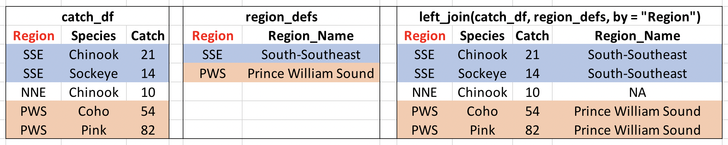
Visualisation of our left_join
First, let’s read in the region definitions data table and select only the columns we want. Note that I have piped my read.csv result into a select call, creating a tidy chunk that reads and selects the data that we need.
region_defs <- read.csv(url("https://knb.ecoinformatics.org/knb/d1/mn/v2/object/df35b.303.1",
                            method = "libcurl"),
                        stringsAsFactors = FALSE) %>%
    select(code, mgmtArea)

head(region_defs)
## code mgmtArea
## 1 GSE Unallocated Southeast Alaska
## 2 NSE Northern Southeast Alaska
## 3 SSE Southern Southeast Alaska
## 4 YAK Yakutat
## 5 PWSmgmt Prince William Sound Management Area
## 6 BER Bering River Subarea Copper River SubareaIf you examine the region_defs data.frame, you’ll see that the column names don’t exactly match the image above. If the names of the key columns are not the same, you can explicitly specify which are the key columns in the left and right side as shown below:
catch_joined <- left_join(catch_clean, region_defs, by = c("Region" = "code"))

head(catch_joined)
## Region Year species catch mgmtArea
## 1 SSE 1886 Chinook 0 Southern Southeast Alaska
## 2 SSE 1887 Chinook 0 Southern Southeast Alaska
## 3 SSE 1888 Chinook 0 Southern Southeast Alaska
## 4 SSE 1889 Chinook 0 Southern Southeast Alaska
## 5 SSE 1890 Chinook 0 Southern Southeast Alaska
## 6 SSE 1891 Chinook 0 Southern Southeast AlaskaNotice that I have deviated from our usual pipe syntax (although it does work here!) because I prefer to see the data.frames that I am joining side by side in the syntax.
Another way you can do this join is to use rename to change the column name code to Region in the region_defs data.frame, and run the left_join this way:
region_defs <- region_defs %>%
  rename(Region = code, Region_Name = mgmtArea)

catch_joined <- left_join(catch_clean, region_defs, by = c("Region"))

head(catch_joined)
Now our catches have the auxiliary information from the region definitions file alongside them. Note: dplyr provides a complete set of joins: inner, left, right, full, semi, anti, not just left_join.
11.13 separate() and unite()
separate() and its complement, unite() allow us to easily split a single column into numerous (or numerous into a single). This can come in really handle when we have a date column and we want to group by year or month. Let’s make a new data.frame with fake data to illustrate this:
dates_df <- data.frame(date = c("5/24/1930",
                                "5/25/1930",
                                "5/26/1930",
                                "5/27/1930",
                                "5/28/1930"),
                       stringsAsFactors = FALSE)

dates_df %>%
  separate(date, c("month", "day", "year"), "/")
## month day year
## 1 5 24 1930
## 2 5 25 1930
## 3 5 26 1930
## 4 5 27 1930
## 5 5 28 1930- Exercise: Split the
citycolumn in the followingdata.frameintocityandstate_codecolumns:
cities_df <- data.frame(city = c("Juneau AK",
                                 "Sitka AK",
                                 "Anchorage AK"),
                        stringsAsFactors = FALSE)

# Write your solution here
unite() does just the reverse of separate():
dates_df %>%
  separate(date, c("month", "day", "year"), "/") %>%
  unite(date, month, day, year, sep = "/")
## date
## 1 5/24/1930
## 2 5/25/1930
## 3 5/26/1930
## 4 5/27/1930
## 5 5/28/1930- Exercise: Use
unite()on your solution above to combine thecities_dfback to its original form with just one column,city:
# Write your solution here11.14 Summary
We just ran through the various things we can do with dplyr and tidyr but if you’re wondering how this might look in a real analysis. Let’s look at that now:
catch_original <- read.csv(url("https://knb.ecoinformatics.org/knb/d1/mn/v2/object/df35b.302.1", method = "libcurl"),
                  stringsAsFactors = FALSE)
region_defs <- read.csv(url("https://knb.ecoinformatics.org/knb/d1/mn/v2/object/df35b.303.1", method = "libcurl"),
                        stringsAsFactors = FALSE) %>%
    select(code, mgmtArea)

mean_region <- catch_original %>%
  select(-All, -notesRegCode) %>%
  gather(species, catch, -Region, -Year) %>%
  mutate(catch = ifelse(catch == "I", 1, catch)) %>%
  mutate(catch = as.integer(catch)*1000) %>%
  group_by(Region) %>%
  summarize(mean_catch = mean(catch)) %>%
  left_join(region_defs, by = c("Region" = "code"))

head(mean_region)
## # A tibble: 6 x 3
## Region mean_catch mgmtArea
## <chr> <dbl> <chr>
## 1 ALU 40384. Aleutian Islands Subarea
## 2 BER 16373. Bering River Subarea Copper River Subarea
## 3 BRB 2709796. Bristol Bay Management Area
## 4 CHG 315487. Chignik Management Area
## 5 CKI 683571. Cook Inlet Management Area
## 6 COP 179223. Copper River Subarea